Vector Database and Semantic Search Engine
Why Traditional Search Falls Short
Think about the last time a search engine returned results that were technically correct but completely useless. You searched for “how to stop a running process” and got results about marathon training. That’s the classic failure of keyword-based search—it matches words, not meaning.
Traditional databases excel at exact lookups: find the row where id = 42. But when you ask “what articles are similar to this one?” or “find products that feel like cozy winter evenings”, structured queries break down completely. This is the gap that vector databases and semantic search were built to close.
Phase 1: Data Ingestion
Every semantic search system starts with a corpus—documents, product descriptions, support tickets, code snippets, or any unstructured content you want to make searchable.
Ingestion Isn’t Just Loading Data
Raw data rarely arrives search-ready. During ingestion, content is cleaned, normalized, and split into digestible units called chunks. Chunking strategy matters enormously. Chunk too broadly and your embeddings lose precision; chunk too narrowly and they lose context.
A common heuristic is 100–256 tokens per chunk, with a small overlap between adjacent chunks to preserve sentence continuity across boundaries. Each chunk is stored alongside its metadata—source URL, timestamp, author, category—so that when it surfaces in search results, it carries enough context to be actionable.
Ingestion Pipeline Components
- Connectors: Pull data from S3, databases, APIs, or file systems
- Parsers: Extract clean text from PDFs, HTML, Markdown, and DOCX
- Chunkers: Split text into semantically coherent segments
- Metadata extractors: Tag each chunk with provenance and filtering fields
At scale, ingestion pipelines are typically asynchronous, running as background jobs that feed a message queue before downstream processing kicks off.
Phase 2: Embedding Generation
This is where the magic begins. An embedding model transforms each text chunk into a high-dimensional numerical vector—a list of floating-point numbers, typically 768 to 3072 dimensions depending on the model.
What Does a Vector Actually Represent?
Think of embedding space as a giant multidimensional map where meaning determines location. Semantically similar texts land close together; unrelated ones drift far apart. The sentence “How do I restart a container?” and “Steps to reboot a Docker instance” map to nearly identical coordinates, even though they share zero words.
This is the core insight that makes semantic search possible.
Choosing an Embedding Model
| Model | Dimensions | Best For |
|---|---|---|
text-embedding-3-small (OpenAI) | 1536 | General-purpose text |
text-embedding-3-large (OpenAI) | 3072 | High-precision retrieval |
all-MiniLM-L6-v2 (Sentence Transformers) | 384 | Lightweight, local deployment |
nomic-embed-text | 768 | Open-source, strong performance |
One critical rule: the same model must be used for both indexing and querying. Mixing models produces meaningless distance comparisons—like measuring in kilometers and miles on the same map.
Batch Processing for Scale
Generating embeddings one-by-one is impractical at scale. Production systems batch chunks together and call the embedding API or local model in parallel, taking care to respect rate limits and manage memory efficiently.
Phase 3: Vector Storage
Once embeddings are generated, they need a home. This is where the vector database enters the picture.
What Makes Vector Databases Different
Relational databases store rows and index them with B-trees, optimized for exact lookups. Vector databases store embeddings and index them with algorithms designed for approximate nearest neighbor (ANN) search—finding vectors that are close to a query vector, not identical to it.
Popular vector database options include:
- Pinecone – Fully managed, serverless, production-grade
- Weaviate – Open-source with built-in embedding and hybrid search
- Qdrant – High-performance Rust-based engine
- Milvus – Distributed, cloud-native architecture
- pgvector – Vector search extension for PostgreSQL
Each chunk is stored as a record containing its vector, the original text, and metadata fields. The metadata is critical for filtered search—for example, retrieving only documents from the last 30 days, or only articles in a specific category.
Storage Schema Example
{
  "id": "chunk_001",
  "vector": [0.021, -0.087, 0.445, ...],
  "text": "Steps to reboot a Docker instance without data loss...",
  "metadata": {
    "source": "docs/containers.md",
    "category": "Infrastructure",
    "created_at": "2026-01-15"
  }
}
Phase 4: Indexing
Storing millions of vectors is one challenge. Searching them in milliseconds is another. This is what the indexing phase solves.
The Approximate Nearest Neighbor Problem
A brute-force similarity search—comparing a query vector against every stored vector—is accurate but catastrophically slow at scale. For 10 million vectors at 1536 dimensions, that’s billions of floating-point operations per query.
ANN index structures trade a small amount of recall for enormous speed gains.
HNSW: The Dominant Algorithm
Hierarchical Navigable Small Worlds (HNSW) is the workhorse of modern vector search. It builds a layered graph where each node connects to its nearest neighbors. Search navigates from coarse upper layers down to precise lower layers, finding approximate nearest neighbors orders of magnitude faster than brute force.
Key HNSW tuning parameters:
M– Number of connections per node (higher = better recall, more memory)ef_construction– Build-time search depth (higher = better index quality, slower indexing)ef_search– Query-time search depth (tunable per request)
Other notable algorithms include IVF (Inverted File Index), which clusters vectors into buckets and searches only relevant clusters, and ScaNN from Google, optimized for maximum throughput on large corpora.
Phase 5: Query Processing
A user types a search query. Here’s what happens in the next 50–200 milliseconds.
Query Pipeline
- Query embedding: The search string is passed through the same embedding model used at index time, producing a query vector.
- ANN search: The vector database runs an approximate nearest neighbor search, returning the top-k most similar chunks (typically k = 10–50).
- Metadata filtering: Pre-filters or post-filters narrow results by metadata fields before or after the vector search.
- Deduplication: Overlapping chunks from the same source document are collapsed into single results.
Pre-filter vs Post-filter
Metadata filtering strategy affects both accuracy and speed. Pre-filtering restricts the search space before the ANN algorithm runs, which is faster but can reduce recall if the filtered subset is small. Post-filtering runs the full vector search then prunes results—better recall, but potentially wastes compute on records that get discarded.
Most production systems default to pre-filtering and fall back to post-filtering when the filtered set is too small to produce meaningful results.
Phase 6: Ranking and Re-ranking
The initial ANN results are ordered by vector similarity, but similarity alone isn’t always the best signal for relevance. Enter re-ranking.
Why Re-rank?
ANN search retrieves semantically related content efficiently, but it’s an approximation. A cross-encoder re-ranker—a model that jointly encodes the query and each candidate result—produces more accurate relevance scores at the cost of higher compute.
The standard two-stage pattern is:
Query → ANN Retrieval (top 50) → Cross-Encoder Re-ranker → Final Results (top 5–10)The retriever acts as a fast, approximate filter. The re-ranker acts as a precise, expensive judge applied only to the shortlist.
Hybrid Search: Combining Semantic and Keyword
Pure semantic search struggles with exact queries: serial numbers, proper nouns, product codes, or highly specific technical terms. The solution is hybrid search, which blends vector similarity scores with traditional keyword (BM25) scores.
The combined ranking is typically computed with Reciprocal Rank Fusion (RRF)—a simple, parameter-free formula that merges two ranked lists without requiring tuning. Most modern vector databases (Weaviate, Qdrant, Elasticsearch) support hybrid search natively.
Putting It All Together
Here’s the end-to-end data flow for a production semantic search system:
Raw Content
    ↓
[ Ingestion & Chunking ]
    ↓
[ Embedding Model ] → High-dimensional vectors
    ↓
[ Vector Database ]
    ↓ ← HNSW Index
[ ANN Search + Metadata Filtering ]
    ↓
[ Re-ranker (optional) ]
    ↓
Ranked Results
Each phase is independently scalable. Embedding generation can be horizontally scaled with worker pools. Vector storage can be sharded across nodes. Re-ranking can be cached for popular queries.
Real-World Considerations
Embedding Drift
Models improve over time. When you upgrade your embedding model, all existing vectors become incompatible with new query vectors. This requires a full re-indexing run—regenerating embeddings for every document. Build your ingestion pipeline with re-indexing in mind from day one.
Latency Budgets
Semantic search introduces new latency sources that keyword search doesn’t have: embedding API calls and ANN index traversal. For P99 latency targets under 200ms, consider caching embeddings for common queries, co-locating the embedding model with the vector database, and using a smaller, faster embedding model for real-time paths.
Cost at Scale
Embedding APIs charge per token. At 10 million documents averaging 500 tokens each, that’s 5 billion tokens just for the initial index—plus ongoing costs as content is added or updated. Evaluate open-source embedding models deployed on dedicated hardware for high-volume workloads.
Conclusion: The Infrastructure Behind Intelligent Search
Vector databases and semantic search represent a step-change in how applications handle information retrieval. The shift from matching words to matching meaning unlocks use cases that were previously impractical: conversational search, similar-item discovery, RAG pipelines, and anomaly detection.
The six phases—ingestion, embedding, storage, indexing, querying, and ranking—each have their own tradeoffs and failure modes. Mastering them individually is straightforward. Getting the full pipeline to perform reliably under real production load is where the real engineering begins.
The teams building on this infrastructure today are laying the groundwork for the next generation of AI-native products. Start with a well-structured ingestion pipeline, choose your embedding model deliberately, and let the architecture evolve from there. 🔍